idopNetwork_vignette

library(idopNetwork)
backup_options <- options()
#load pre-computered results
test_result = idopNetwork:::test_result

About

idopNetwork is packed as a cartographic tool that performs power curve fitting, classification, variable selection, microbial abundance decomposition, and network visualization based on microbial 16S rRNA gene sequencing metadata.

For complete details on the use and execution of this protocol, please refer to Chen et al and Cao et al.

1. Input data

Before running idopNetwork, user need to provide datasets, and they should be cleaned and merged to exactly the same format of the example data.

1.1 gut microbe OTUs data

Microbe Operational taxonomic unit dataset must have first column as IDs for microbes.

data("gut_microbe")
View(gut_microbe)

name	GQ_UC1	GQ_UC3	GQ_UC4	GQ_UC5
Escherichia_coli	176	1701	28506	177
Arthrobacter_oxydans	3	215	1578	1
Ruminococcus_gnavus	744	0	4	733
Bacteroides_plebeius	271	4401	7	8394
Bacteroides_pyogenes	0	15	0	0
Clostridium_tertium	305	1	1	270
Bacteroides_stercoris	24	0	0	11
Flavisolibacter_ginsengisoli	0	123	831	0
Bacteroides_massiliensis	0	6098	6	0
Prevotella_heparinolytica	0	6	0	0

1.2 mustard microbe OTUs data

data("mustard_microbe")
View(mustard_microbe)

	ID	8_0149.leaf	8_0157.leaf	8_0158.leaf	8_0160.leaf
2	OTU_1	3	2	59	268
3	OTU_2	8	13	1890	44
4	OTU_3	5485	3302	4522	6581
5	OTU_4	42	351	7	4
6	OTU_5	16	2002	24	43
7	OTU_6	1645	1170	10636	31686
8	OTU_7	4050	4094	13	66
9	OTU_8	6	282	124	27
10	OTU_9	102	5	10	18
11	OTU_10	25	1393	35	19

	JAM_E4.leaf	8_0149.root	8_0157.root	8_0158.root	8_0160.root
2	7	28861	122	1	9
3	4	11618	19	14	1894
4	4981	481	755	17914	15998
5	622	862	1072	11	103
6	10014	447	758	19	289
7	577	1010	490	25030	29443
8	2233	13	5575	26	64
9	19	3348	36	33	46
10	362	6269	228	2	459
11	3071	4	6454	6	234

2. power curve fitting

The first major step in our idopNetwork reconstruction is to fit allometric growth curves to the data using the power function. This is easily done by using the related function power_fit. This function needs cleaned dataset as input and will return fitted OTUs for given dataset. Then the fitted output with original dataset can be transfer into function power_equation_plot for quick visualization

df = data_cleaning(gut_microbe)

result1 = power_equation_fit(df)

power_equation_plot(result1)

3. Functional clustering

In this step we implement the power equation into functional clustering to detect different microbial modules. If after clustering there are still too many microbes within a certain module for network reconstruction, we can rerun functional clustering to further classify this module into distinct submodules.

3.1 mean curve

we fit mean vector of each cluster center by power equation(assume k=3)

matplot(t(power_equation(x = 1:30, matrix(c(2,1,3,0.2,0.5,-0.5),nrow = 3, ncol = 2))), 
        type = "l",
        xlab = "time", 
        ylab = "population")
legend("topright", 
       c("cluster 1", "cluster 2", "cluster 3"), 
       lty = c(1,2,3), 
       col = c(1,2,3), 
       box.lwd = 0)

3.2 covariance matrix

we fit covariance matrix of multivariate normal distribution with SAD1, it can be showed as

get_SAD1_covmatrix(c(2,0.5), n = 5)
#>      [,1]  [,2]  [,3]  [,4]  [,5]
#> [1,] 0.25  0.50  1.00  2.00  4.00
#> [2,] 0.50  1.25  2.50  5.00 10.00
#> [3,] 1.00  2.50  5.25 10.50 21.00
#> [4,] 2.00  5.00 10.50 21.25 42.50
#> [5,] 4.00 10.00 21.00 42.50 85.25

3.3 initial parameters

we can check initial parameters (k=4)

get_par_int(X = log10(df+1), k = 4, times = as.numeric(log10(colSums(df)+1)))
#> Error in nls(y ~ a * x^b, start = list(a = a, b = b), control = nls.control(maxiter = 1000,  : 
#>   number of iterations exceeded maximum of 1000
#> Error in nls(y ~ a * x^b, start = list(a = a, b = b), control = nls.control(maxiter = 1000,  : 
#>   number of iterations exceeded maximum of 1000
#> Error in nls(y ~ a * x^b, start = list(a = a, b = b), control = nls.control(maxiter = 1000,  : 
#>   number of iterations exceeded maximum of 1000
#> Error in nls(y ~ a * x^b, start = list(a = a, b = b), control = nls.control(maxiter = 1000,  : 
#>   number of iterations exceeded maximum of 1000
#> Error in nls(y ~ a * x^b, start = list(a = a, b = b), control = nls.control(maxiter = 1000,  : 
#>   number of iterations exceeded maximum of 1000
#> Error in nls(y ~ a * x^b, start = list(a = a, b = b), control = nls.control(maxiter = 1000,  : 
#>   number of iterations exceeded maximum of 1000
#> Error in nls(y ~ a * x^b, start = list(a = a, b = b), control = nls.control(maxiter = 1000,  : 
#>   number of iterations exceeded maximum of 1000
#> $initial_cov_params
#> [1] 0.50000 1.09618
#> 
#> $initial_mu_params
#>                 a           b
#> [1,] 1.222931e+15 -21.7299294
#> [2,] 2.241187e-35  50.4618037
#> [3,] 1.275766e+01  -0.8462029
#> [4,] 1.930699e+02  -3.6047139
#> 
#> $initial_probibality
#> 
#>          1          2          3          4 
#> 0.24590164 0.27868852 0.06557377 0.40983607

#use kmeans to get initial centers
tmp = kmeans(log10(df+1),4)$centers
tmp2 = power_equation_fit(tmp, trans = NULL)
power_equation_plot(tmp2, label = NULL,n = 4)

3.4 functional clustering (power-equation,SAD1)

idopNetowrk already wrapped the mean curve modelling, covariance matrix modelling and likelihood ratio calculation into a function fun_clu().

options(max.print = 10)
fun_clu(result1$original_data, k = 3, iter.max = 5)
#> Error in nls(y ~ a * x^b, start = list(a = a, b = b), control = nls.control(maxiter = 1000,  : 
#>   number of iterations exceeded maximum of 1000
#> initial  value 1224.701250 
#> final  value 1224.701250 
#> converged
#> 
#>  iter = 1 
#>  Log-Likelihood =  1229.444 
#> initial  value 1228.240624 
#> final  value 1228.240624 
#> converged
#> 
#>  iter = 2 
#>  Log-Likelihood =  1225.461 
#> initial  value 1224.705979 
#> final  value 1224.705979 
#> converged
#> 
#>  iter = 3 
#>  Log-Likelihood =  1226.112 
#> initial  value 1225.588016 
#> final  value 1225.588016 
#> converged
#> 
#>  iter = 4 
#>  Log-Likelihood =  1224.793 
#> initial  value 1224.655751 
#> final  value 1224.655751 
#> converged
#> 
#>  iter = 5 
#>  Log-Likelihood =  1224.97 
#> initial  value 1224.822485 
#> final  value 1224.822485 
#> converged
#> 
#>  iter = 6 
#>  Log-Likelihood =  1227.894
#> $cluster_number
#> [1] 3
#> 
#> $Log_likelihodd
#> [1] 1227.894
#> 
#> $AIC
#> [1] 2475.787
#> 
#> $BIC
#> [1] 2494.499
#> 
#> $cov_par
#> [1] 0.500000 1.098059
#> 
#> $mu_par
#>              [,1]       [,2]
#> [1,] 2.161219e-15  21.401464
#> [2,] 4.804131e+01  -1.686739
#> [3,] 2.210693e+16 -23.629600
#> 
#> $probibality
#> [1] 0.57603917 0.07110126 0.35285957
#> 
#> $omega
#>               [,1]         [,2]         [,3]
#>  [1,] 2.536304e-01 3.140715e-04 7.460555e-01
#>  [2,] 4.400950e-01 2.237826e-04 5.596812e-01
#>  [3,] 5.594828e-01 1.463402e-06 4.405157e-01
#>  [ reached getOption("max.print") -- omitted 45 rows ]
#> 
#> $cluster
#>      MC_UC3 MC_UC4 YZJC_UC3 GQ_UC3 ZC_UC3 MC_UC2 GQ_UC1 GQ_UC4 HJC_UC3 ZC_UC4
#>      HJC_UC1 HJC_UC4 HC_UC2 ZC_UC1 HC_UC4 JJC_UC2 HJC_UC2 MC_UC1 GQ_UC5 ZC_UC5
#>      apply(omega, 1, which.max)
#>  [ reached 'max' / getOption("max.print") -- omitted 48 rows ]
#> 
#> $cluster2
#>      MC_UC3 MC_UC4 YZJC_UC3 GQ_UC3 ZC_UC3 MC_UC2 GQ_UC1 GQ_UC4 HJC_UC3 ZC_UC4
#>      HJC_UC1 HJC_UC4 HC_UC2 ZC_UC1 HC_UC4 JJC_UC2 HJC_UC2 MC_UC1 GQ_UC5 ZC_UC5
#>      apply(omega, 1, which.max)
#>  [ reached 'max' / getOption("max.print") -- omitted 48 rows ]
#> 
#>  [ reached getOption("max.print") -- omitted 2 entries ]

Usually we use multithread to calcuation k = 2-n and then to decide best k , fun_clu_BIC uses BIC to select best cluster number by default.

result2 = fun_clu_parallel(result1$original_data, start = 2, end = 5)

best.k = which.min(sapply( result2 , "[[" , 'BIC' )) + 1 #skipped k = 1
best.k
#> [1] 7

fun_clu_BIC(result = result2)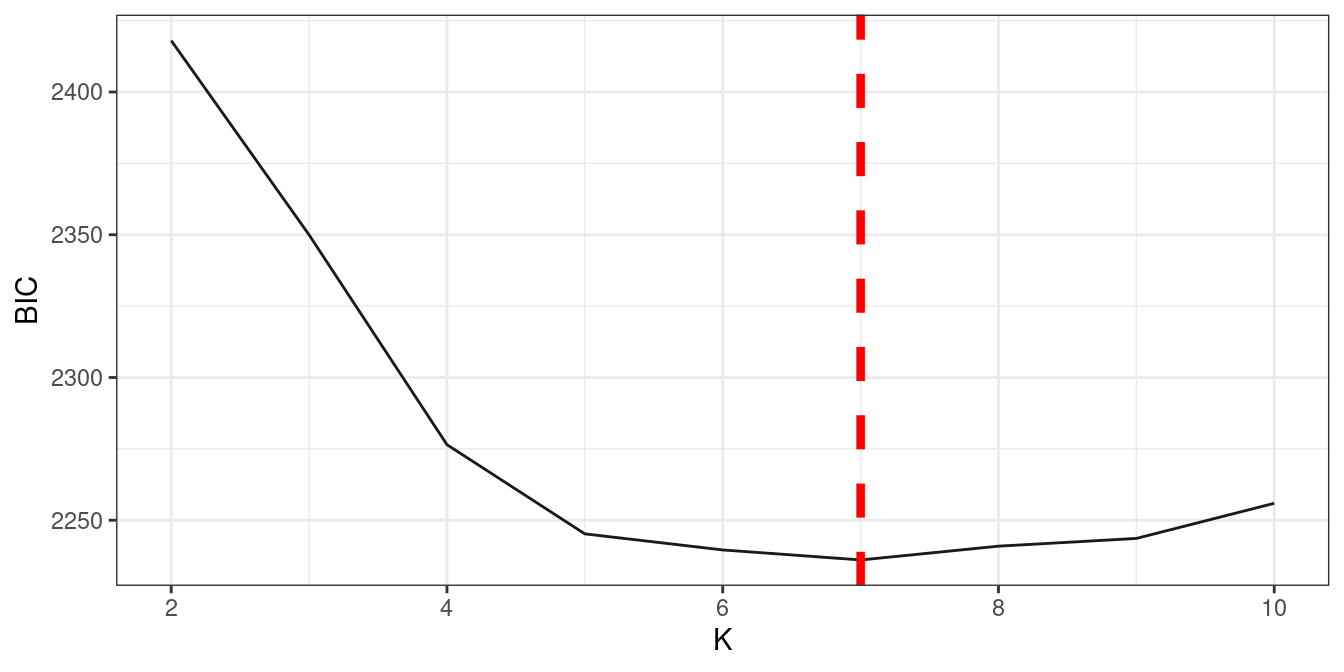


#we can direct give other k value
fun_clu_plot(result = result2, best.k = best.k)

3.5 bi-functional clustering (power-equation,biSAD1)

In this part we select part of mustard data for demonstration purpose.

data("mustard_microbe")
df2 = data_cleaning(mustard_microbe, x = 160)

res_l = power_equation_fit(df2[,1:5]
res_r = power_equation_fit(df2[,89:95])
res1 = data_match(result1 = res_l, result2 = res_r)

res2 = bifun_clu_parallel(data1 = res1$dataset1$original_data, 
                          data2 = res1$dataset2$original_data,
                          Time1 = res1$dataset1$Time, 
                          Time2 = res1$dataset2$Time,
                          start = 2, 
                          end = 10, 
                          thread = 9,
                          iter.max = 10)

res2 = bifun_clu_parallel(data1 = res1$dataset1$original_data, 
                          data2 = res1$dataset2$original_data,
                          Time1 = res1$dataset1$Time, 
                          Time2 = res1$dataset2$Time,
                          start = 2, 
                          end = 10, 
                          thread = 9,
                          iter.max = 10)

fun_clu_BIC(result = res2)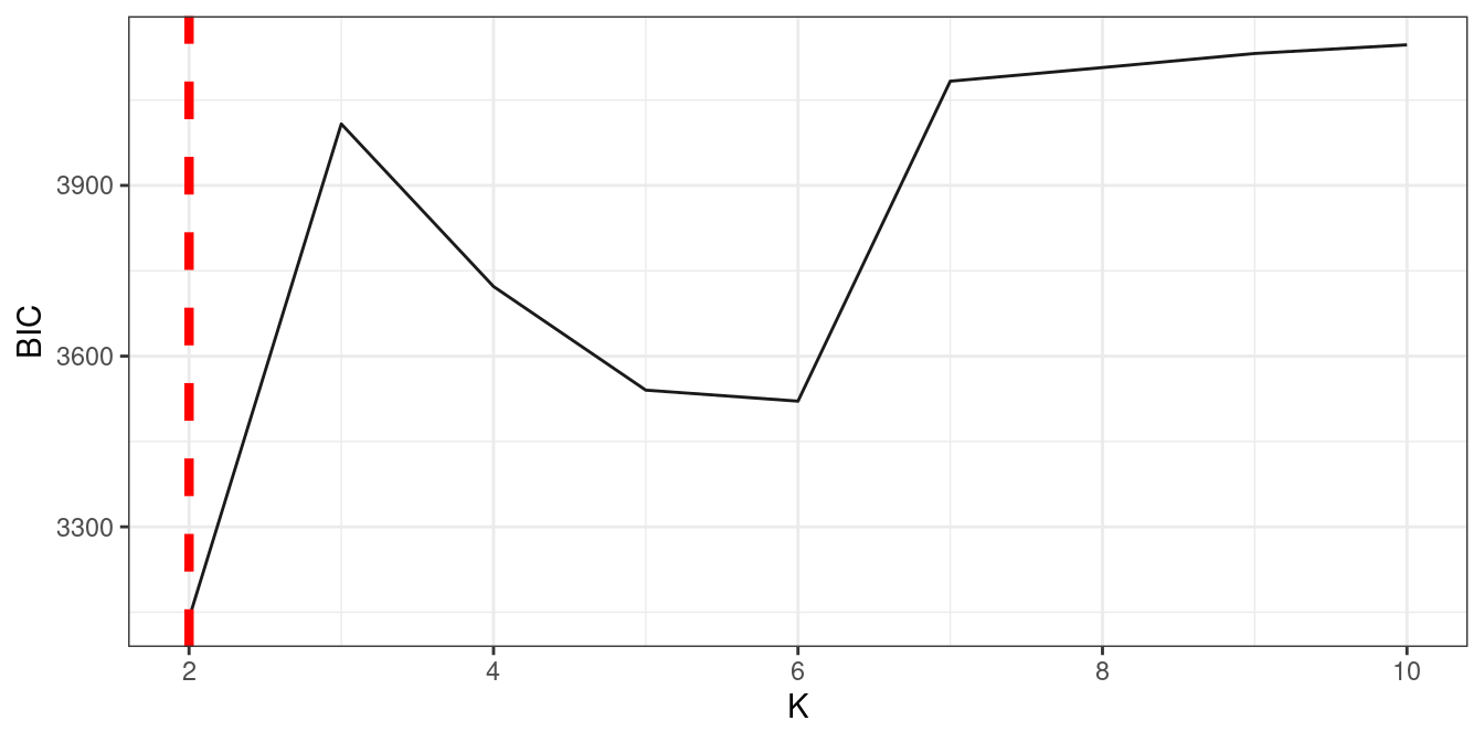


#we can set best.k directly
bifun_clu_plot(result = res2, best.k = 3, color1 = "#C060A1", color2 = "#59C1BD")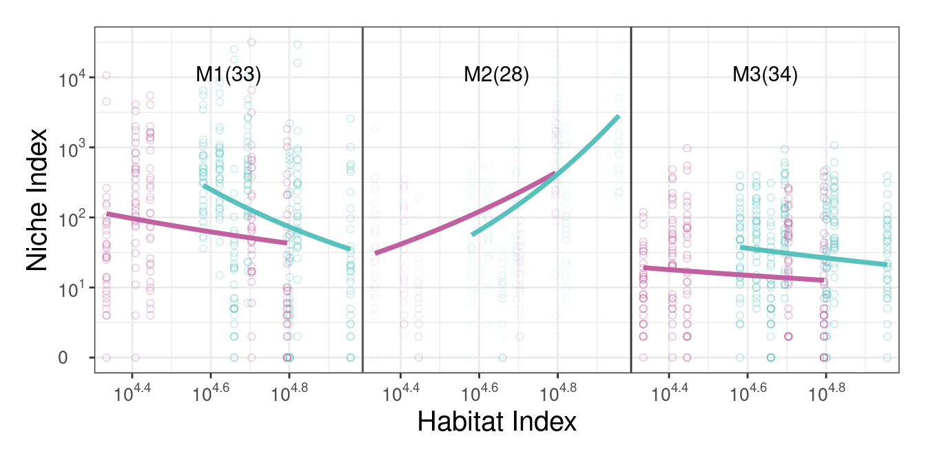

3.6 sub-clustering

Sometimes a module is still too large for network reconstruction, which is determined by Dunbar’s number, we can further cluster it into sub-modules.

res3 = bifun_clu_convert(res2, best.k = 3)
large.module = order(sapply(res3$a$Module.all,nrow))[5]

res_suba = fun_clu_select(result_fit = res1$dataset1, result_funclu = res3$a, i = large.module)
res_subb = fun_clu_select(result_fit = res1$dataset2, result_funclu = res3$b, i = large.module)
dfsuba_l = power_equation_fit(res_suba$original_data)
dfsubb_r = power_equation_fit(res_subb$original_data)
ressub1 = data_match(result1 = dfsuba_l, result2 = dfsubb_r)
ressub2 = bifun_clu_parallel(data1 = ressub1$dataset1$original_data, 
                             data2 = ressub1$dataset2$original_data,
                             Time1 = ressub1$dataset1$Time, 
                             Time2 = ressub1$dataset2$Time, 
                             start = 2, 
                             end = 5, 
                             iter.max = 3)

ressub2 = test_result$d2_subcluster

fun_clu_BIC(result = ressub2)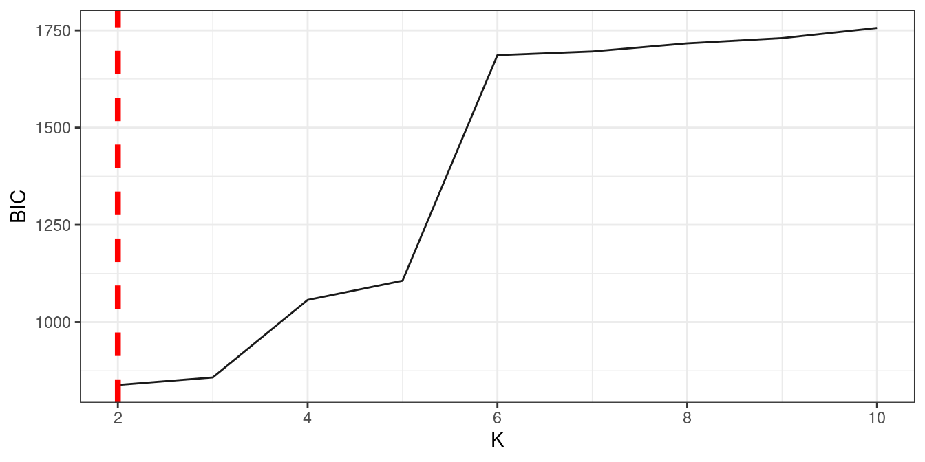

bifun_clu_plot(result = ressub2, best.k = 2, color1 = "#C060A1", color2 = "#59C1BD", degree = 1)

4. LASSO-based variable selection

idopNetwork implements a LASSO-based procedure to choose a small set of the most significant microbes/module that links with a given microbes/modules. get_interaction()return a compound list contain the target microbe/module name, the most relevant Modules/microbes names and the coefficients.

4.1 For Modules

result3 = fun_clu_convert(result2,best.k = best.k)
df.module = result3$original_data
get_interaction(df.module,1)
#> $ind.name
#> [1] "M1"
#> 
#> $dep.name
#> [1] "M5"
#> 
#> $coefficient
#> [1] 5.964078

4.2 For Microbes

#we can the microbial relationship in Module1
df.M1 = result3$Module.all$`1`
get_interaction(df.M1,1)
#> Warning: Option grouped=FALSE enforced in cv.glmnet, since < 3 observations per
#> fold

#> Warning: Option grouped=FALSE enforced in cv.glmnet, since < 3 observations per
#> fold

#> Warning: Option grouped=FALSE enforced in cv.glmnet, since < 3 observations per
#> fold
#> $ind.name
#> [1] "Arthrobacter_oxydans"
#> 
#> $dep.name
#> [1] "Fusobacterium_necrophorum"
#> 
#> $coefficient
#> [1] 0.08263525

5 qdODE solving

qdODE system is build based on variable selection results, it has unique ability to decompose the observed module/microbe abundance level into its independent component and dependent component, which can be used for inferring idopNetwork.

5.1 solving qdODE between modules

options(max.print = 10)
# first we test solving a qdODE
module.relationship = lapply(1:best.k, function(c)get_interaction(df.module,c))
ode.test = qdODE_all(result = result3, relationship = module.relationship, 1, maxit = 100)
#> iter   10 value 0.004336
#> final  value 0.000002 
#> converged
# we can view the result
qdODE_plot_base(ode.test)

# then we solve all qdODEs
ode.module = qdODE_parallel(result3)

qdODE_plot_all(ode.module)

5.2 solving qdODE within a module

result_m1 = fun_clu_select(result_fit = result1, result_funclu = result3, i = 1)
ode.M1 = qdODE_parallel(result_m1)

qdODE_plot_all(ode.M1)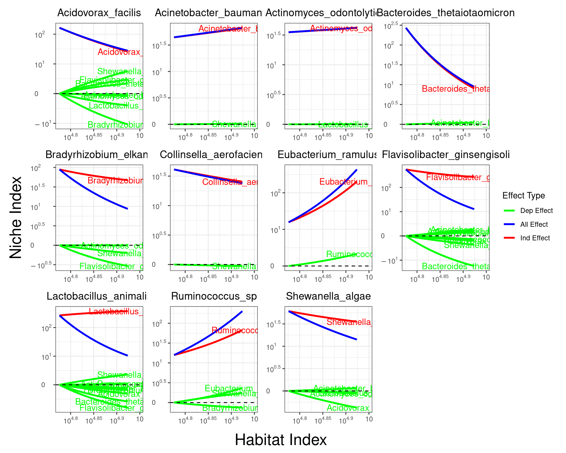

6 idopNetwork reconstruction

The final step of this guide is to visualization the multilayer network, and our package provide network_plot function to easily draw our idopNetwork. We can simply plug previous qdODE results into network_conversion function, and it will convert qdODE result for network visualization

6.1 network between modules

net_module = lapply(ode.module$ode_result, network_conversion)
network_plot(net_module, title = "Module Network")

6.2 network within a module

net_m1 = lapply(ode.M1$ode_result, network_conversion)
network_plot(net_m1, title = "M1 Network")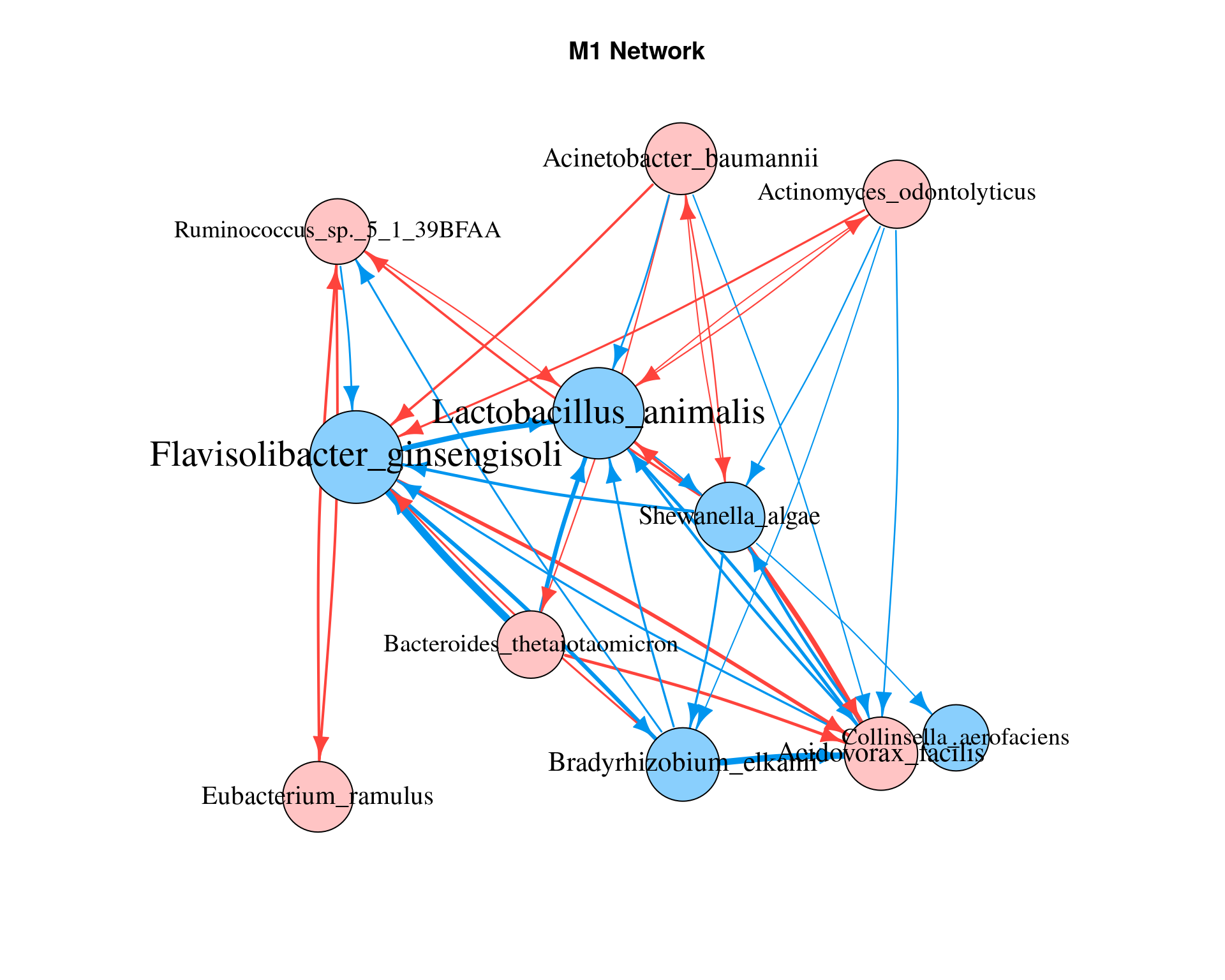

6.3 network comparison

mustard_module_a = qdODE_parallel(res3$a) 
mustard_module_b = qdODE_parallel(res3$b) 

res_m1a = fun_clu_select(result_fit = res1$dataset1, result_funclu = res3$a, i = 3)
res_m1b = fun_clu_select(result_fit = res1$dataset2, result_funclu = res3$b, i = 3)
mustard_M1a = qdODE_parallel(res_m1a)
mustard_M1b = qdODE_parallel(res_m1b)

mustard_m_a <- lapply(mustard_module_a$ode_result, network_conversion)
mustard_m_b <- lapply(mustard_module_b$ode_result, network_conversion)

#set seed to make same random layout
layout(matrix(c(1,2),1,2,byrow=TRUE))
set.seed(1)
network_plot(mustard_m_a, title = "Module Network a")
set.seed(1)
network_plot(mustard_m_b, title = "Module Network b")

result_m1a = fun_clu_select(result_fit = res1$dataset1, result_funclu = res3$a, i = 1)
result_m1b = fun_clu_select(result_fit = res1$dataset2, result_funclu = res3$b, i = 1)
ode.m1a = qdODE_parallel(result_m1a, thread = 16)
ode.m1b = qdODE_parallel(result_m1b, thread = 16)

net_m1a = lapply(ode.m1a$ode_result, network_conversion)
net_m1b = lapply(ode.m1b$ode_result, network_conversion)

#set seed to make same random layout
layout(matrix(c(1,2),1,2,byrow=TRUE))
set.seed(1)
network_plot(net_m1a, title = "Module1 a")
set.seed(1)
network_plot(net_m1b, title = "Module1 b")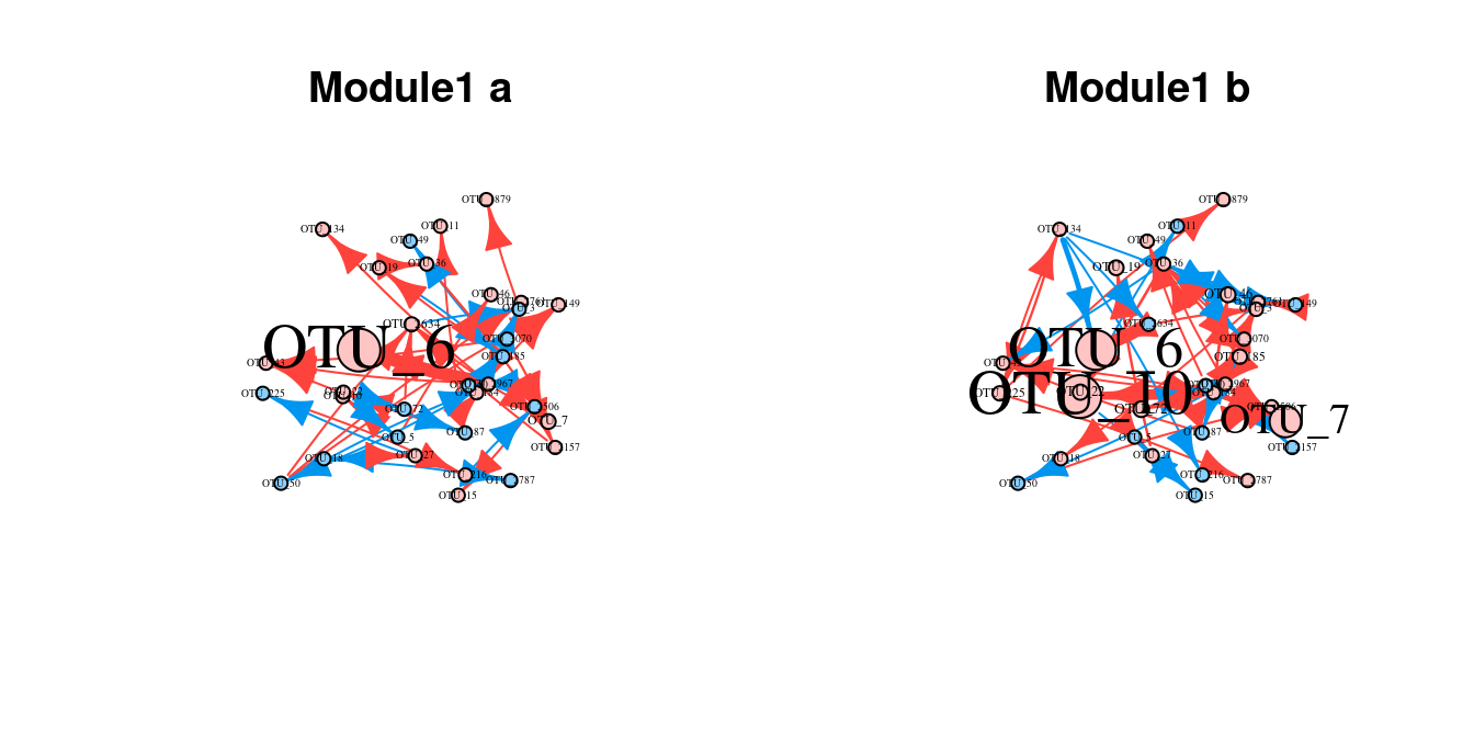

Troubleshooting

object “LL.next” not found
This happens when parameters optimization failure, try rerun cluster.

plot failure when using fun_clu_plot() or bifun_clu_plot()
This often happens when bad initial parameters is given and some cluster is lost, try rerun cluster or use a smaller k.

Session info

sessionInfo()
#> R version 4.3.0 (2023-04-21)
#> Platform: x86_64-pc-linux-gnu (64-bit)
#> Running under: Ubuntu 22.04.2 LTS
#> 
#> Matrix products: default
#> BLAS:   /usr/lib/x86_64-linux-gnu/openblas-pthread/libblas.so.3 
#> LAPACK: /usr/lib/x86_64-linux-gnu/openblas-pthread/libopenblasp-r0.3.20.so;  LAPACK version 3.10.0
#> 
#> locale:
#>  [1] LC_CTYPE=C.UTF-8       LC_NUMERIC=C           LC_TIME=C.UTF-8       
#>  [4] LC_COLLATE=C.UTF-8     LC_MONETARY=C.UTF-8    LC_MESSAGES=C.UTF-8   
#>  [7] LC_PAPER=C.UTF-8       LC_NAME=C              LC_ADDRESS=C          
#> [10] LC_TELEPHONE=C         LC_MEASUREMENT=C.UTF-8 LC_IDENTIFICATION=C   
#> 
#> time zone: UTC
#> tzcode source: system (glibc)
#> 
#> attached base packages:
#> [1] stats     graphics  grDevices utils     datasets  methods   base     
#> 
#> other attached packages:
#> [1] idopNetwork_0.1.2
#> 
#> loaded via a namespace (and not attached):
#>  [1] sass_0.4.6           utf8_1.2.3           shape_1.4.6         
#>  [4] stringi_1.7.12       lattice_0.21-8       digest_0.6.31       
#>  [7] magrittr_2.0.3       evaluate_0.21        grid_4.3.0          
#> [10] iterators_1.0.14     mvtnorm_1.2-1        fastmap_1.1.1       
#> [13] plyr_1.8.8           foreach_1.5.2        rprojroot_2.0.3     
#> [16] jsonlite_1.8.5       glmnet_4.1-7         Matrix_1.5-4        
#> [19] deSolve_1.35         survival_3.5-5       purrr_1.0.1         
#> [22] fansi_1.0.4          scales_1.2.1         codetools_0.2-19    
#> [25] textshaping_0.3.6    jquerylib_0.1.4      cli_3.6.1           
#> [28] rlang_1.1.1          munsell_0.5.0        splines_4.3.0       
#> [31] withr_2.5.0          cachem_1.0.8         yaml_2.3.7          
#> [34] tools_4.3.0          parallel_4.3.0       reshape2_1.4.4      
#> [37] polynom_1.4-1        memoise_2.0.1        colorspace_2.1-0    
#> [40] ggplot2_3.4.2        orthopolynom_1.0-6.1 vctrs_0.6.2         
#> [43] R6_2.5.1             lifecycle_1.0.3      stringr_1.5.0       
#> [46] fs_1.6.2             ragg_1.2.5           pkgconfig_2.0.3     
#> [49] desc_1.4.2           pkgdown_2.0.7        pillar_1.9.0        
#> [52] bslib_0.4.2          gtable_0.3.3         glue_1.6.2          
#> [55] Rcpp_1.0.10          systemfonts_1.0.4    highr_0.10          
#> [58] xfun_0.39            tibble_3.2.1         knitr_1.43          
#> [61] farver_2.1.1         patchwork_1.1.2      htmltools_0.5.5     
#> [64] igraph_1.4.3         labeling_0.4.2       rmarkdown_2.22      
#> [67] compiler_4.3.0

Ang Dong

06/07/2023